5 Alpha diversities
Alpha diversity measures are used to identify within individual taxa richness and evenness. The commonly used metrics/indices are Shannon, Inverse Simpson, Simpson, Gini, Observed and Chao1. These indices do not take into account the phylogeny of the taxa identified in sequencing. Phylogenetic diversity (Faith’s PD) uses phylogenetic distance to calculate the diversity of a given sample.
It is important to note that, alpha diversity indices are sensitive to noise that is inherent to application of polymerase chain reaction and the sequencing errors.
One has to consider the sequencing depth (how much of the taxa have been sampled) for each sample. If there is a large difference, then it is important to normalize the samples to equal sampling depth. First, we look at the sampling depth (no. of reads per sample).
Load packages
library(microbiome) # data analysis and visualisation
library(phyloseq) # also the basis of data object. Data analysis and visualisation
library(microbiomeutilities) # some utility tools
library(RColorBrewer) # nice color options
library(ggpubr) # publication quality figures, based on ggplot2
library(DT) # interactive tables in html and markdown
library(data.table) # alternative to data.frame
library(dplyr) # data handling
The data for tutorial is stored as *.rds file in the R project phyobjects folder.
We will use the filtered phyloseq object from Set-up and Pre-processing section.
ps1 <- readRDS("./phyobjects/ps.ng.tax.rds")

# use print option to see the data saved as phyloseq object.

print(ps1)
## phyloseq-class experiment-level object
## otu_table() OTU Table: [ 4710 taxa and 474 samples ]
## sample_data() Sample Data: [ 474 samples by 30 sample variables ]
## tax_table() Taxonomy Table: [ 4710 taxa by 6 taxonomic ranks ]
## phy_tree() Phylogenetic Tree: [ 4710 tips and 4709 internal nodes ]## Min. 1st Qu. Median Mean 3rd Qu. Max.
## 2458 6436 8188 9836 10306 115023As is evident there is a large difference in the number of reads. Minimum is 2458 and maximum is 115023!! There is a ~47X difference!
We can plot the rarefaction curve for the observed ASVs in the entire data set. This is a way to check how has the richness captured in the sequencing effort.
otu_tab <- t(abundances(ps1))
p <- vegan::rarecurve(otu_tab,
                      step = 50, label = FALSE,
                      sample = min(rowSums(otu_tab),
                                   col = "blue", cex = 0.6))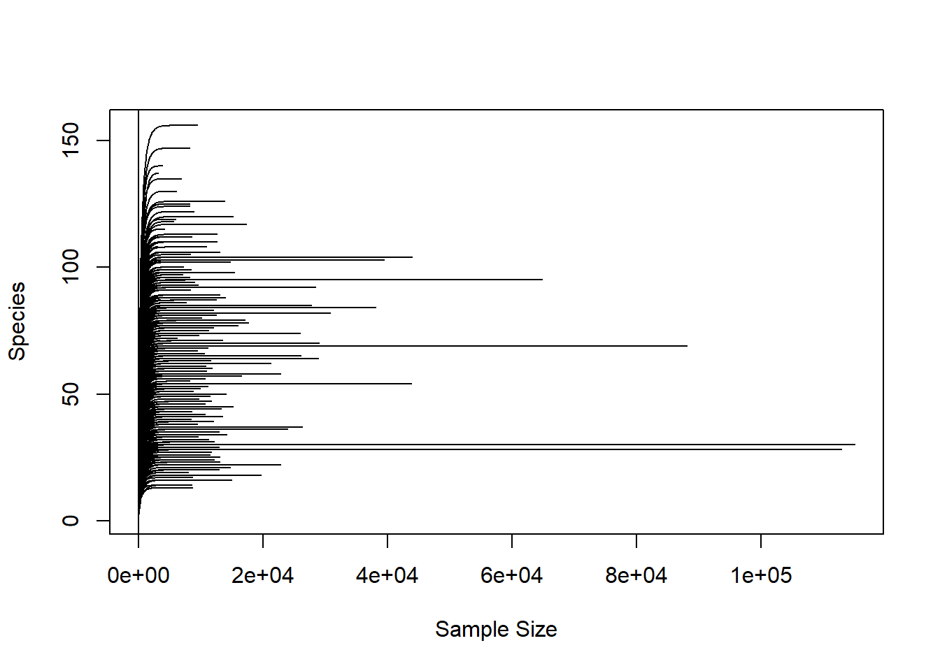
Almost all samples are reaching a plateau and few samples have high number of reads and high number of ASVs.
Since we are comparing different body sites, some are expected to have low bacterial load.
We will normalize to the lowest depth of at least 2458 reads to keep maximum samples for our anlaysis. This can be varied to remove samples with lower sequencing depth. This decision will depend on the research question being addressed.
Note: At the end of this section, we look at relationship between reads per samples and diversity metrics.
5.1 Equal sample sums
set.seed(9242)  # This will help in reproducing the filtering and nomalisation.

ps0.rar <- rarefy_even_depth(ps1, sample.size = 2458)
## You set `rngseed` to FALSE. Make sure you've set & recorded
## the random seed of your session for reproducibility.
## See `?set.seed`## ...## 63OTUs were removed because they are no longer
## present in any sample after random subsampling## ...Check how much data you have now
## phyloseq-class experiment-level object
## otu_table()   OTU Table:         [ 4647 taxa and 474 samples ]
## sample_data() Sample Data:       [ 474 samples by 30 sample variables ]
## tax_table()   Taxonomy Table:    [ 4647 taxa by 6 taxonomic ranks ]
## phy_tree()    Phylogenetic Tree: [ 4647 tips and 4646 internal nodes ]
The plot below is only for a quick and dirty check for reads per samples.
Quick check taxa prevalence.
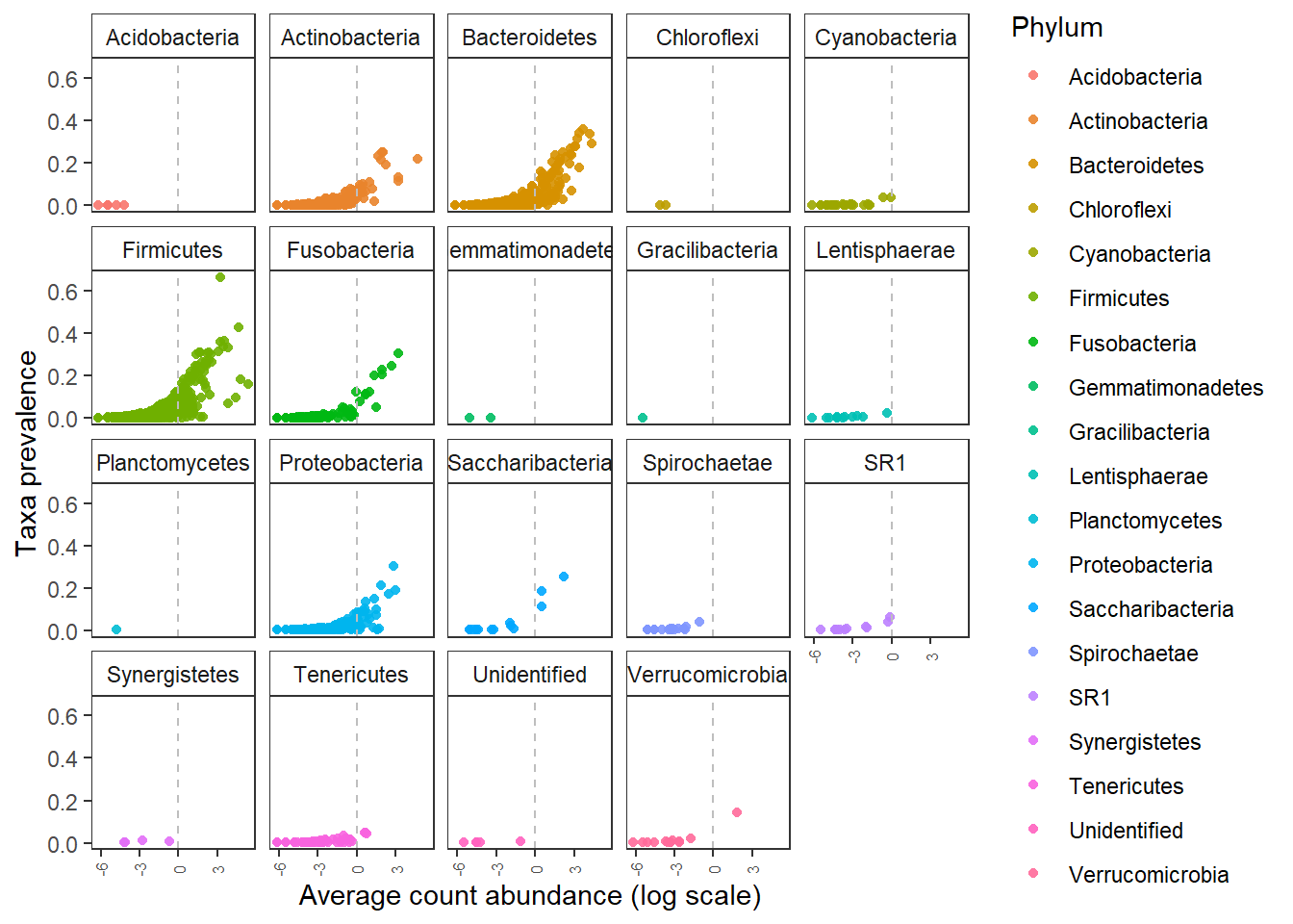
Compare this to taxa prevalence plot from previous section of the tutorial.
Do you see any difference?
5.2 Diversities
5.2.1 Non-phylogenetic diversities
For more diversity indices please refer to Microbiome Package
Let us calculate diversity.
## Observed richness## Other forms of richness## Diversity## Evenness## Dominance## RarityThis is one way to plot the data.
# get the metadata out as seprate object
hmp.meta <- meta(ps0.rar)

# Add the rownames as a new colum for easy integration later.
hmp.meta$sam_name <- rownames(hmp.meta)

# Add the rownames to diversity table
hmp.div$sam_name <- rownames(hmp.div)

# merge these two data frames into one
div.df <- merge(hmp.div,hmp.meta, by = "sam_name")

# check the tables
colnames(div.df)
## [1] "sam_name" "observed"
## [3] "chao1" "diversity_inverse_simpson"
## [5] "diversity_gini_simpson" "diversity_shannon"
## [7] "diversity_fisher" "diversity_coverage"
## [9] "evenness_camargo" "evenness_pielou"
## [11] "evenness_simpson" "evenness_evar"
## [13] "evenness_bulla" "dominance_dbp"
## [15] "dominance_dmn" "dominance_absolute"
## [17] "dominance_relative" "dominance_simpson"
## [19] "dominance_core_abundance" "dominance_gini"
## [21] "rarity_log_modulo_skewness" "rarity_low_abundance"
## [23] "rarity_rare_abundance" "BarcodeSequence"
## [25] "LinkerPrimerSequence" "run_prefix"
## [27] "body_habitat" "body_product"
## [29] "body_site" "bodysite"
## [31] "dna_extracted" "elevation"
## [33] "env" "env_biome"
## [35] "env_feature" "env_material"
## [37] "env_package" "geo_loc_name"
## [39] "host_common_name" "host_scientific_name"
## [41] "host_subject_id" "host_taxid"
## [43] "latitude" "longitude"
## [45] "physical_specimen_location" "physical_specimen_remaining"
## [47] "psn" "public"
## [49] "sample_type" "scientific_name"
## [51] "sequencecenter" "title"
## [53] "Description"# Now use this data frame to plot
p <- ggboxplot(div.df,
x = "scientific_name",
y = "diversity_shannon",
fill = "scientific_name",
palette = "jco")
p <- p + rotate_x_text()
print(p)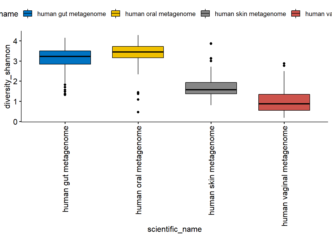
##  [1] "observed"                   "chao1"
##  [3] "diversity_inverse_simpson"  "diversity_gini_simpson"
##  [5] "diversity_shannon"          "diversity_fisher"
##  [7] "diversity_coverage"         "evenness_camargo"
##  [9] "evenness_pielou"            "evenness_simpson"
## [11] "evenness_evar"              "evenness_bulla"
## [13] "dominance_dbp"              "dominance_dmn"
## [15] "dominance_absolute"         "dominance_relative"
## [17] "dominance_simpson"          "dominance_core_abundance"
## [19] "dominance_gini"             "rarity_log_modulo_skewness"
## [21] "rarity_low_abundance"       "rarity_rare_abundance"
## [23] "sam_name"
Alternative way
# convert phyloseq object into a long data format.

div.df2 <- div.df[, c("scientific_name", "diversity_inverse_simpson", "diversity_gini_simpson", "diversity_shannon", "diversity_fisher", "diversity_coverage")]

# the names are not pretty. we can replace them

colnames(div.df2) <- c("Location", "Inverse Simpson", "Gini-Simpson", "Shannon", "Fisher", "Coverage")

# check
colnames(div.df2)
## [1] "Location" "Inverse Simpson" "Gini-Simpson" "Shannon"
## [5] "Fisher" "Coverage"## Using Location as id variables## Location variable value
## 1 human gut metagenome Inverse Simpson 28.66520
## 2 human gut metagenome Inverse Simpson 30.34355
## 3 human oral metagenome Inverse Simpson 15.73401
## 4 human oral metagenome Inverse Simpson 16.22464
## 5 human gut metagenome Inverse Simpson 18.81490
## 6 human gut metagenome Inverse Simpson 20.88379The diversity indices are stored under column named variable.
# Now use this data frame to plot
p <- ggboxplot(div_df_melt, x = "Location", y = "value",
              fill = "Location",
              palette = "jco",
              legend= "right",
              facet.by = "variable",
              scales = "free")

p <- p + rotate_x_text()
# we will remove the x axis lables

p <- p + rremove("x.text")
p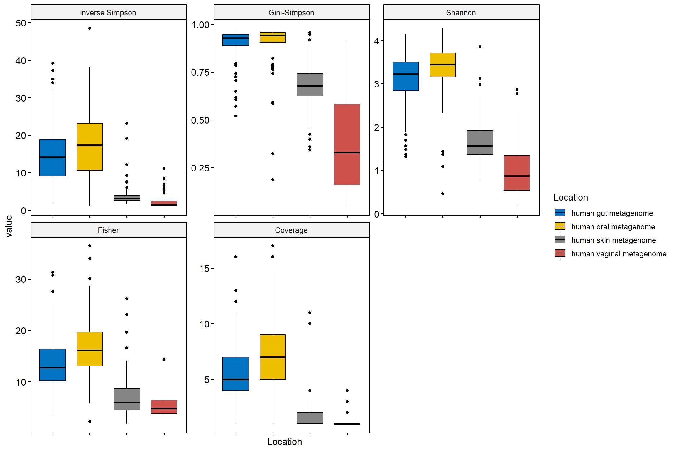
lev <- levels(div_df_melt$Location) # get the variables

# make a pairwise list that we want to compare.
L.pairs <- combn(seq_along(lev), 2, simplify = FALSE, FUN = function(i) lev[i])

pval <- list(
  cutpoints = c(0, 0.0001, 0.001, 0.01, 0.05, 0.1, 1),
  symbols = c("****", "***", "**", "*", "n.s")
)

p2 <- p + stat_compare_means(
  comparisons = L.pairs,
  label = "p.signif",
  symnum.args = list(
    cutpoints = c(0, 0.0001, 0.001, 0.01, 0.05, 0.1, 1),
    symbols = c("****", "***", "**", "*", "n.s")
  )
)

print(p2)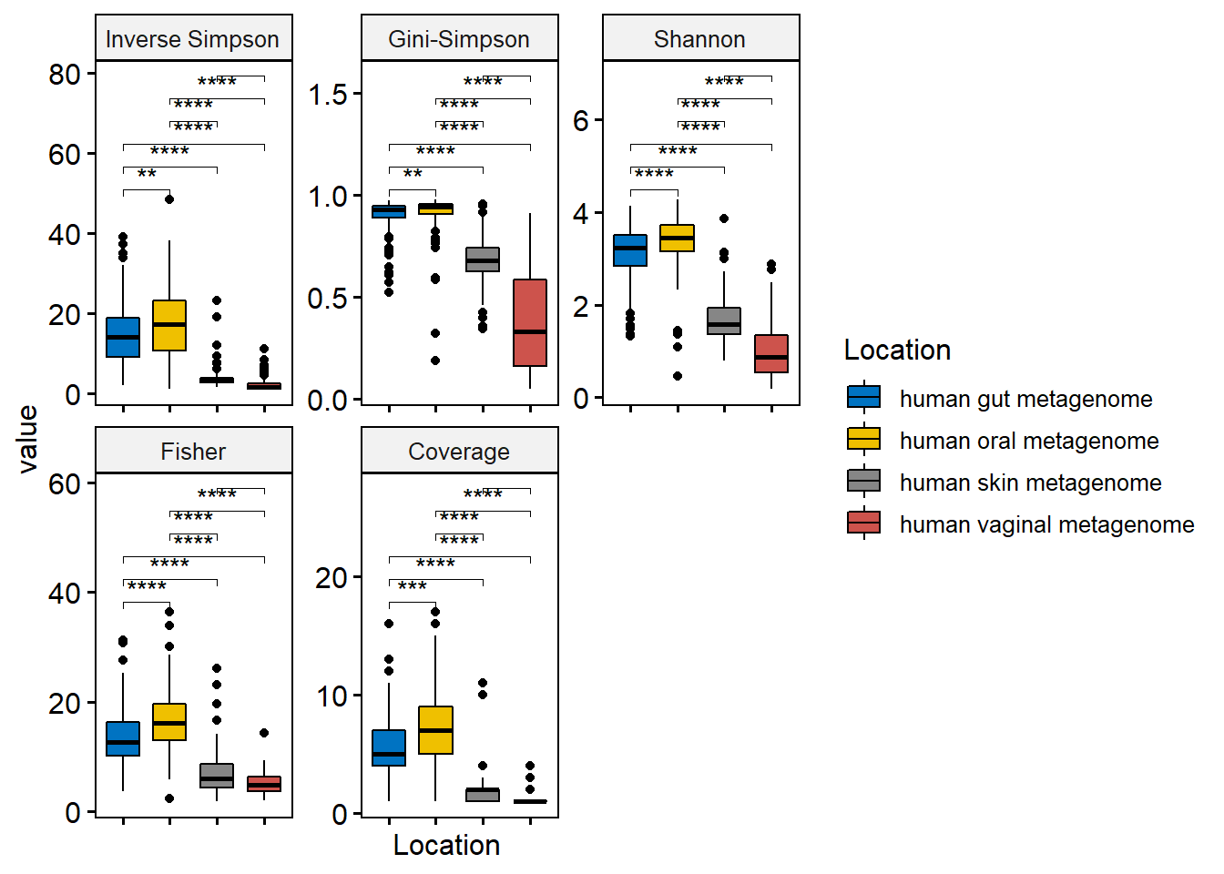
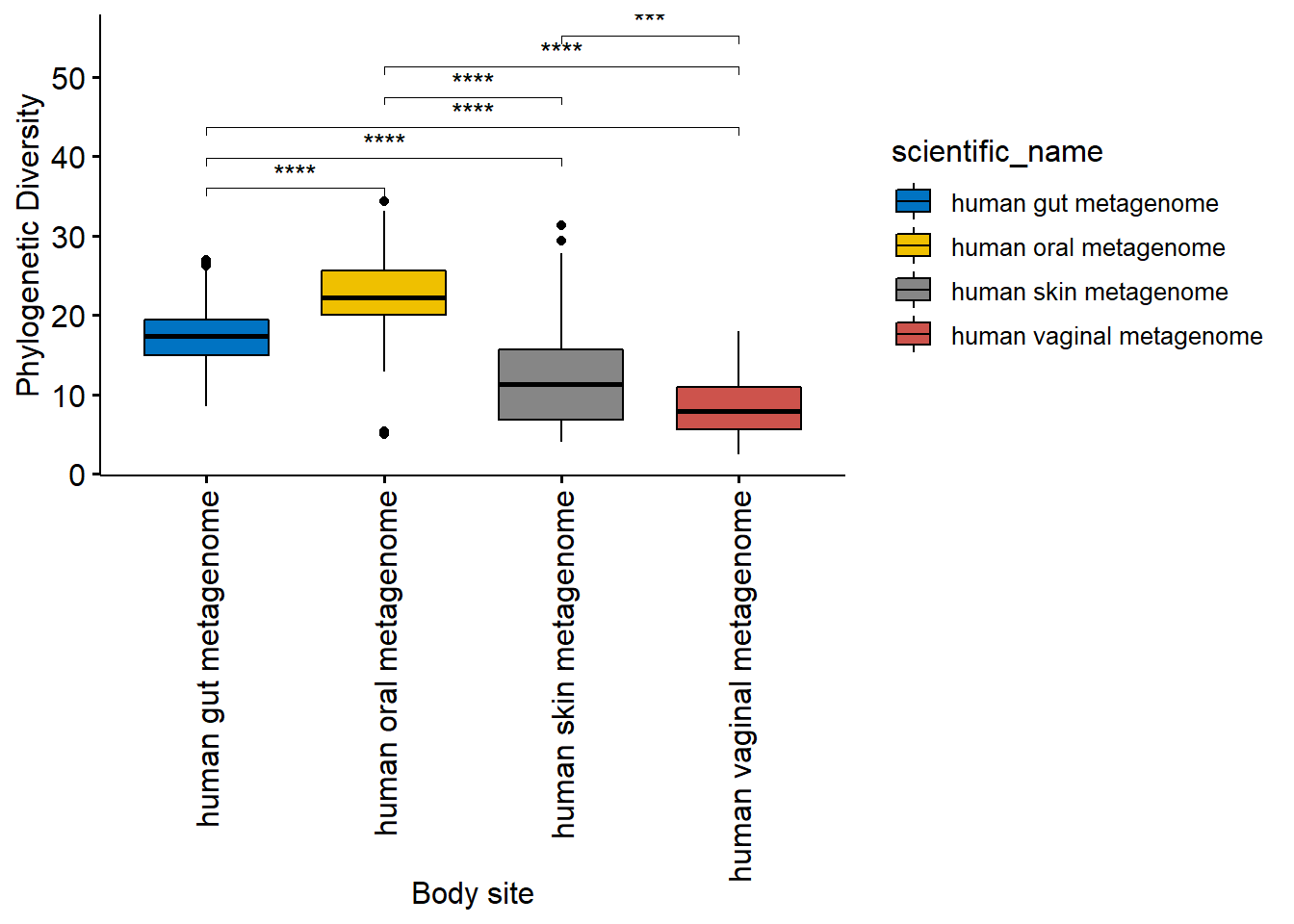
5.2.2 Phylogenetic diversity
Phylogenetic diversity is calculated using the picante package.
library(picante)

ps0.rar.asvtab <- as.data.frame(ps0.rar@otu_table)

ps0.rar.tree <- ps0.rar@phy_tree

# hmp.meta from previous code chunks

# We first need to check if the tree is rooted or not

ps0.rar@phy_tree
##
## Phylogenetic tree with 4647 tips and 4646 internal nodes.
##
## Tip labels:
## 9410494158, 9410494576, 9410491420, 9410491569, 9410491595, 9410491783, ...
##
## Rooted; includes branch lengths.# it is a rooted tree
df.pd <- pd(t(ps0.rar.asvtab), ps0.rar.tree,include.root=T) # t(ou_table) transposes the table for use in picante and the tre file comes from the first code chunck we used to read tree file (see making a phyloseq object section).
datatable(df.pd)now we need to plot PD. Check above how to get the metadata file from a phyloseq object.
# now we need to plot PD

# We will add the results of PD to this file and then plot.

hmp.meta$Phylogenetic_Diversity <- df.pd$PD
Plot
pd.plot <- ggboxplot(hmp.meta,
  x = "scientific_name",
  y = "Phylogenetic_Diversity",
  fill = "scientific_name",
  palette = "jco",
  ylab = "Phylogenetic Diversity",
  xlab = "Body site",
  legend = "right"
)
pd.plot <- pd.plot + rotate_x_text()

pd.plot + stat_compare_means(
  comparisons = L.pairs,
  label = "p.signif",
  symnum.args = list(
    cutpoints = c(0, 0.0001, 0.001, 0.01, 0.05, 0.1, 1),
    symbols = c("****", "***", "**", "*", "n.s")
  )
)
NOTE:
There are arguments both for and against the use of rarefying to equal library size.
The application of normalization method will depend on the type of research question. It is always good to check if there is a correlation between increasing library sizes and richness. Observed ASVs and Phylogenetic diversity can be affected by library sizes. It is always good to check for this before making a choice.
## Observed richness## Other forms of richness## Diversity## Evenness## Dominance## Raritylib.div2 <- richness(ps1)
# let us add nmber of total reads/samples
lib.div$ReadsPerSample <- sample_sums(ps1)
lib.div$Observed <- lib.div2$observed
colnames(lib.div)## [1] "observed" "chao1"
## [3] "diversity_inverse_simpson" "diversity_gini_simpson"
## [5] "diversity_shannon" "diversity_fisher"
## [7] "diversity_coverage" "evenness_camargo"
## [9] "evenness_pielou" "evenness_simpson"
## [11] "evenness_evar" "evenness_bulla"
## [13] "dominance_dbp" "dominance_dmn"
## [15] "dominance_absolute" "dominance_relative"
## [17] "dominance_simpson" "dominance_core_abundance"
## [19] "dominance_gini" "rarity_log_modulo_skewness"
## [21] "rarity_low_abundance" "rarity_rare_abundance"
## [23] "ReadsPerSample" "Observed"We will use ggscatter function from ggpubr package to visualze.
p1 <- ggscatter(lib.div, "diversity_shannon", "ReadsPerSample") +
  stat_cor(method = "pearson")

p2 <- ggscatter(lib.div, "diversity_inverse_simpson", "ReadsPerSample",
  add = "loess"
) +
  stat_cor(method = "pearson")

p3 <- ggscatter(lib.div, "Observed", "ReadsPerSample",
  add = "loess") +
  stat_cor(
    method = "pearson",
    label.x = 100,
    label.y = 50000
  )

ggarrange(p1, p2, p3, ncol = 2, nrow = 2)
## `geom_smooth()` using formula 'y ~ x'
## `geom_smooth()` using formula 'y ~ x'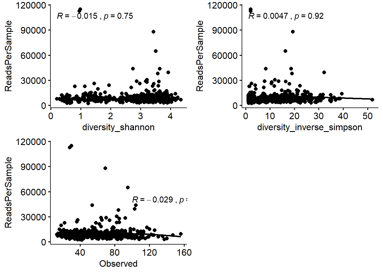
## R version 3.6.3 (2020-02-29)
## Platform: x86_64-w64-mingw32/x64 (64-bit)
## Running under: Windows 10 x64 (build 18363)
##
## Matrix products: default
##
## locale:
## [1] LC_COLLATE=English_Netherlands.1252  LC_CTYPE=English_Netherlands.1252
## [3] LC_MONETARY=English_Netherlands.1252 LC_NUMERIC=C
## [5] LC_TIME=English_Netherlands.1252
##
## attached base packages:
## [1] stats     graphics  grDevices utils     datasets  methods   base
##
## other attached packages:
##  [1] picante_1.8.1               nlme_3.1-145
##  [3] vegan_2.5-6                 lattice_0.20-40
##  [5] permute_0.9-5               ape_5.3
##  [7] dplyr_0.8.5                 data.table_1.12.8
##  [9] DT_0.12                     ggpubr_0.2.5
## [11] magrittr_1.5                RColorBrewer_1.1-2
## [13] microbiomeutilities_0.99.02 microbiome_1.8.0
## [15] ggplot2_3.3.0               phyloseq_1.30.0
##
## loaded via a namespace (and not attached):
##  [1] Biobase_2.46.0      viridis_0.5.1       tidyr_1.0.2
##  [4] jsonlite_1.6.1      viridisLite_0.3.0   splines_3.6.3
##  [7] foreach_1.4.8       assertthat_0.2.1    stats4_3.6.3
## [10] yaml_2.2.1          ggrepel_0.8.2       pillar_1.4.3
## [13] glue_1.3.2          digest_0.6.25       ggsignif_0.6.0
## [16] XVector_0.26.0      colorspace_1.4-1    cowplot_1.0.0
## [19] htmltools_0.4.0     Matrix_1.2-18       plyr_1.8.6
## [22] pkgconfig_2.0.3     pheatmap_1.0.12     bookdown_0.18
## [25] zlibbioc_1.32.0     purrr_0.3.3         scales_1.1.0
## [28] Rtsne_0.15          tibble_2.1.3        mgcv_1.8-31
## [31] farver_2.0.3        IRanges_2.20.2      withr_2.1.2
## [34] BiocGenerics_0.32.0 survival_3.1-11     crayon_1.3.4
## [37] evaluate_0.14       MASS_7.3-51.5       tools_3.6.3
## [40] lifecycle_0.2.0     stringr_1.4.0       Rhdf5lib_1.8.0
## [43] S4Vectors_0.24.3    munsell_0.5.0       cluster_2.1.0
## [46] ggsci_2.9           Biostrings_2.54.0   ade4_1.7-15
## [49] compiler_3.6.3      rlang_0.4.5         rhdf5_2.30.1
## [52] grid_3.6.3          iterators_1.0.12    biomformat_1.14.0
## [55] htmlwidgets_1.5.1   crosstalk_1.1.0.1   igraph_1.2.4.2
## [58] labeling_0.3        rmarkdown_2.1       gtable_0.3.0
## [61] codetools_0.2-16    multtest_2.42.0     reshape2_1.4.3
## [64] R6_2.4.1            gridExtra_2.3       knitr_1.28
## [67] stringi_1.4.6       parallel_3.6.3      Rcpp_1.0.4
## [70] vctrs_0.2.4         tidyselect_1.0.0    xfun_0.12